分類問題を解く ～分析編～

どうも，筆者です．

決定木による分類

今回は，決定木を用いて分析を行う．使用するコードを以下に示す．

#!/usr/bin/python
# -*- coding: utf-8 -*-

import pandas as pd
import numpy as np
import matplotlib.pyplot as plt
from sklearn.tree import DecisionTreeClassifier

def get_data(target_df):
    X = np.array([target_df['Temperature'].tolist(), target_df['Humidity'].tolist()], dtype=np.float64).T
    y = np.array(target_df['Status'].tolist(), dtype=np.int32)
    return X, y

#
# 決定境界プロット関数
#
def plot_decision_regions(x, y, model, resolution=0.01):
    ## 2変数の入力データの最小値から最大値まで引数resolutionの幅でメッシュを描く
    x1_min, x1_max = x[:, 0].min()-1, x[:, 0].max()+1
    x2_min, x2_max = x[:, 1].min()-1, x[:, 1].max()+1
    x1_mesh, x2_mesh = np.meshgrid(np.arange(x1_min, x1_max, resolution),
                                   np.arange(x2_min, x2_max, resolution))

    ## メッシュデータ全部を学習モデルで分類
    z = model.predict(np.array([x1_mesh.ravel(), x2_mesh.ravel()]).T)
    z = z.reshape(x1_mesh.shape)

    ## メッシュデータと分離クラスを使って決定境界を描いている
    fig, ax = plt.subplots(figsize=(10, 10))
    ax.contourf(x1_mesh, x2_mesh, z, alpha=0.3, cmap='jet')
    ax.set_xlim(x1_mesh.min(), x1_mesh.max())
    ax.set_ylim(x2_mesh.min(), x2_mesh.max())

    ax.scatter(x=x[y==0, 0],y=x[y==0, 1],c='blue', cmap='jet')
    ax.scatter(x=x[y==1, 0],y=x[y==1, 1],c='red', cmap='jet')
    ax.set_xlabel('Temperature')
    ax.set_ylabel('Humidity')
    return fig, ax

if __name__ == '__main__':
    train_df = pd.read_csv('train_data.csv', header=0)
    test_df = pd.read_csv('test_data.csv', header=0)
    train_X, train_y = get_data(train_df)
    test_X, test_y = get_data(test_df)

    for i in np.arange(10):
        depth = i + 1
        tree = DecisionTreeClassifier(max_depth=depth).fit(train_X, train_y)
        fig, ax = plot_decision_regions(train_X, train_y, tree)
        ax.set_title('Tree Depth {}'.format(depth))
        plt.savefig('result_decisionTree/dtree_train_depth{}.png'.format(depth))
        plt.close(fig)
        print('Depth: {:2d}, Accuracy(train, test): ({}, {})'.format(depth, tree.score(train_X, train_y), tree.score(test_X, test_y)))

得られた結果のうち，木の深さが1と10のものを以下に示す．

木の深さ: 1

木の深さ: 10

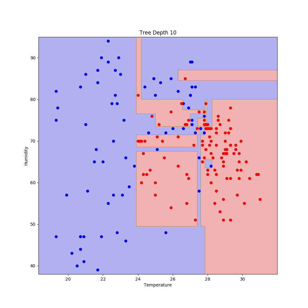
過学習気味である．精度を確認する（精度だけでは不十分であるが）．

木の深さ	精度（学習用データ）	精度（テスト用データ）
1	0.8206521739130435	0.8152173913043478
2	0.8804347826086957	0.8586956521739131
3	0.8858695652173914	0.8586956521739131
4	0.8913043478260869	0.8913043478260869
5	0.9239130434782609	0.8695652173913043
6	0.9347826086956522	0.8913043478260869
7	0.9619565217391305	0.8804347826086957
8	0.9728260869565217	0.8586956521739131
9	0.9782608695652174	0.8695652173913043
10	0.9836956521739131	0.8695652173913043

一番精度が良いものは，木の深さが4の時である．

ランダムフォレストによる分類

続いて，ランダムフォレストによる分類を行う．使用するコードを以下に示す．

#!/usr/bin/python
# -*- coding: utf-8 -*-

import pandas as pd
import numpy as np
import matplotlib.pyplot as plt
from sklearn.ensemble import RandomForestClassifier

def get_data(target_df):
    X = np.array([target_df['Temperature'].tolist(), target_df['Humidity'].tolist()], dtype=np.float64).T
    y = np.array(target_df['Status'].tolist(), dtype=np.int32)
    return X, y

#
# 決定境界プロット関数
#
def plot_decision_regions(x, y, model, resolution=0.01):
    ## 2変数の入力データの最小値から最大値まで引数resolutionの幅でメッシュを描く
    x1_min, x1_max = x[:, 0].min()-1, x[:, 0].max()+1
    x2_min, x2_max = x[:, 1].min()-1, x[:, 1].max()+1
    x1_mesh, x2_mesh = np.meshgrid(np.arange(x1_min, x1_max, resolution),
                                   np.arange(x2_min, x2_max, resolution))

    ## メッシュデータ全部を学習モデルで分類
    z = model.predict(np.array([x1_mesh.ravel(), x2_mesh.ravel()]).T)
    z = z.reshape(x1_mesh.shape)

    ## メッシュデータと分離クラスを使って決定境界を描いている
    fig, ax = plt.subplots(figsize=(10, 10))
    ax.contourf(x1_mesh, x2_mesh, z, alpha=0.3, cmap='jet')
    ax.set_xlim(x1_mesh.min(), x1_mesh.max())
    ax.set_ylim(x2_mesh.min(), x2_mesh.max())

    ax.scatter(x=x[y==0, 0],y=x[y==0, 1],c='blue', cmap='jet')
    ax.scatter(x=x[y==1, 0],y=x[y==1, 1],c='red', cmap='jet')
    ax.set_xlabel('Temperature')
    ax.set_ylabel('Humidity')
    return fig, ax

if __name__ == '__main__':
    train_df = pd.read_csv('train_data.csv', header=0)
    test_df = pd.read_csv('test_data.csv', header=0)
    train_X, train_y = get_data(train_df)
    test_X, test_y = get_data(test_df)

    for est_num in [3, 5, 10, 15, 20]:
        forest = RandomForestClassifier(n_estimators=est_num).fit(train_X, train_y)
        fig, ax = plot_decision_regions(train_X, train_y, forest)
        ax.set_title('Tree Estimators {}'.format(est_num))
        plt.savefig('result_randomForest/rforest_train_est{}.png'.format(est_num))
        plt.close(fig)
        print('Estimators: {:2d}, Accuracy(train, test): ({}, {})'.format(est_num, forest.score(train_X, train_y), forest.score(test_X, test_y)))

得られた結果のうち，決定木の数が10と15のものを以下に示す．

決定木の数: 10

決定木の数: 15

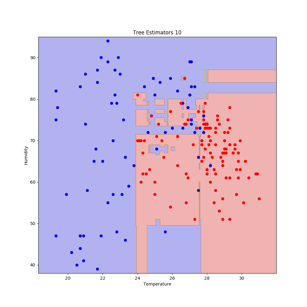
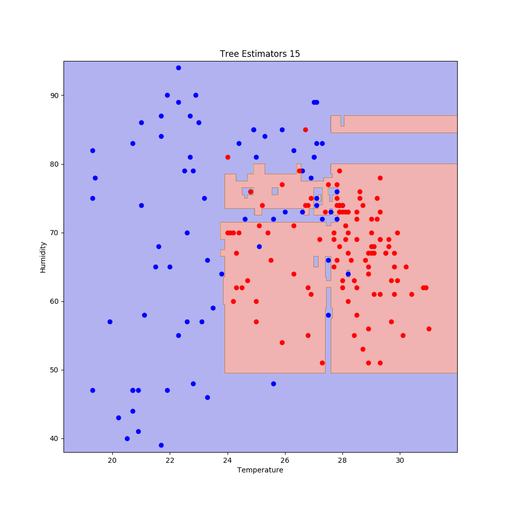
こちらも少し過学習気味である．精度を確認する．

決定木の数	精度（学習用データ）	精度（テスト用データ）
3	0.9456521739130435	0.8913043478260869
5	0.9510869565217391	0.8695652173913043
10	0.9728260869565217	0.8804347826086957
15	0.967391304347826	0.8913043478260869
20	0.9836956521739131	0.8586956521739131

決定木の数が3の時が最も良いが，これは，決定木で推定した場合の精度と変わらない．ランダムフォレストの利点が見いだせない．学習用データとテスト用データの構成が似ているから，これが限界かもしれない．